MATHHX A
\(\newcommand{\footnotename}{footnote}\)
\(\def \LWRfootnote {1}\)
\(\newcommand {\footnote }[2][\LWRfootnote ]{{}^{\mathrm {#1}}}\)
\(\newcommand {\footnotemark }[1][\LWRfootnote ]{{}^{\mathrm {#1}}}\)
\(\let \LWRorighspace \hspace \)
\(\renewcommand {\hspace }{\ifstar \LWRorighspace \LWRorighspace }\)
\(\newcommand {\TextOrMath }[2]{#2}\)
\(\newcommand {\mathnormal }[1]{{#1}}\)
\(\newcommand \ensuremath [1]{#1}\)
\(\newcommand {\LWRframebox }[2][]{\fbox {#2}} \newcommand {\framebox }[1][]{\LWRframebox } \)
\(\newcommand {\setlength }[2]{}\)
\(\newcommand {\addtolength }[2]{}\)
\(\newcommand {\setcounter }[2]{}\)
\(\newcommand {\addtocounter }[2]{}\)
\(\newcommand {\arabic }[1]{}\)
\(\newcommand {\number }[1]{}\)
\(\newcommand {\noalign }[1]{\text {#1}\notag \\}\)
\(\newcommand {\cline }[1]{}\)
\(\newcommand {\directlua }[1]{\text {(directlua)}}\)
\(\newcommand {\luatexdirectlua }[1]{\text {(directlua)}}\)
\(\newcommand {\protect }{}\)
\(\def \LWRabsorbnumber #1 {}\)
\(\def \LWRabsorbquotenumber "#1 {}\)
\(\newcommand {\LWRabsorboption }[1][]{}\)
\(\newcommand {\LWRabsorbtwooptions }[1][]{\LWRabsorboption }\)
\(\def \mathchar {\ifnextchar "\LWRabsorbquotenumber \LWRabsorbnumber }\)
\(\def \mathcode #1={\mathchar }\)
\(\let \delcode \mathcode \)
\(\let \delimiter \mathchar \)
\(\def \oe {\unicode {x0153}}\)
\(\def \OE {\unicode {x0152}}\)
\(\def \ae {\unicode {x00E6}}\)
\(\def \AE {\unicode {x00C6}}\)
\(\def \aa {\unicode {x00E5}}\)
\(\def \AA {\unicode {x00C5}}\)
\(\def \o {\unicode {x00F8}}\)
\(\def \O {\unicode {x00D8}}\)
\(\def \l {\unicode {x0142}}\)
\(\def \L {\unicode {x0141}}\)
\(\def \ss {\unicode {x00DF}}\)
\(\def \SS {\unicode {x1E9E}}\)
\(\def \dag {\unicode {x2020}}\)
\(\def \ddag {\unicode {x2021}}\)
\(\def \P {\unicode {x00B6}}\)
\(\def \copyright {\unicode {x00A9}}\)
\(\def \pounds {\unicode {x00A3}}\)
\(\let \LWRref \ref \)
\(\renewcommand {\ref }{\ifstar \LWRref \LWRref }\)
\( \newcommand {\multicolumn }[3]{#3}\)
\(\require {textcomp}\)
\(\require {colortbl}\)
\(\let \LWRorigcolumncolor \columncolor \)
\(\renewcommand {\columncolor }[2][named]{\LWRorigcolumncolor [#1]{#2}\LWRabsorbtwooptions }\)
\(\let \LWRorigrowcolor \rowcolor \)
\(\renewcommand {\rowcolor }[2][named]{\LWRorigrowcolor [#1]{#2}\LWRabsorbtwooptions }\)
\(\let \LWRorigcellcolor \cellcolor \)
\(\renewcommand {\cellcolor }[2][named]{\LWRorigcellcolor [#1]{#2}\LWRabsorbtwooptions }\)
\(\newcommand {\tothe }[1]{^{#1}}\)
\(\newcommand {\raiseto }[2]{{#2}^{#1}}\)
\(\newcommand {\LWRsiunitxEND }{}\)
\(\def \LWRsiunitxang #1;#2;#3;#4\LWRsiunitxEND {\ifblank {#1}{}{\num {#1}\degree }\ifblank {#2}{}{\num {#2}^{\unicode {x2032}}}\ifblank {#3}{}{\num {#3}^{\unicode {x2033}}}}\)
\(\newcommand {\ang }[2][]{\LWRsiunitxang #2;;;\LWRsiunitxEND }\)
\(\def \LWRsiunitxdistribunit {}\)
\(\newcommand {\LWRsiunitxENDTWO }{}\)
\(\def \LWRsiunitxprintdecimalsubtwo #1,#2,#3\LWRsiunitxENDTWO {\ifblank {#1}{0}{\mathrm {#1}}\ifblank {#2}{}{{\LWRsiunitxdecimal }\mathrm {#2}}}\)
\(\def \LWRsiunitxprintdecimalsub #1.#2.#3\LWRsiunitxEND {\LWRsiunitxprintdecimalsubtwo #1,,\LWRsiunitxENDTWO \ifblank {#2}{}{{\LWRsiunitxdecimal }\LWRsiunitxprintdecimalsubtwo
#2,,\LWRsiunitxENDTWO }}\)
\(\newcommand {\LWRsiunitxprintdecimal }[1]{\LWRsiunitxprintdecimalsub #1...\LWRsiunitxEND }\)
\(\def \LWRsiunitxnumplus #1+#2+#3\LWRsiunitxEND {\ifblank {#2}{\LWRsiunitxprintdecimal {#1}}{\ifblank {#1}{\LWRsiunitxprintdecimal {#2}}{\LWRsiunitxprintdecimal {#1}\unicode
{x02B}\LWRsiunitxprintdecimal {#2}}}\LWRsiunitxdistribunit }\)
\(\def \LWRsiunitxnumminus #1-#2-#3\LWRsiunitxEND {\ifblank {#2}{\LWRsiunitxnumplus #1+++\LWRsiunitxEND }{\ifblank {#1}{}{\LWRsiunitxprintdecimal {#1}}\unicode {x02212}\LWRsiunitxprintdecimal
{#2}\LWRsiunitxdistribunit }}\)
\(\def \LWRsiunitxnumpmmacro #1\pm #2\pm #3\LWRsiunitxEND {\ifblank {#2}{\LWRsiunitxnumminus #1---\LWRsiunitxEND }{\LWRsiunitxprintdecimal {#1}\unicode {x0B1}\LWRsiunitxprintdecimal
{#2}\LWRsiunitxdistribunit }}\)
\(\def \LWRsiunitxnumpm #1+-#2+-#3\LWRsiunitxEND {\ifblank {#2}{\LWRsiunitxnumpmmacro #1\pm \pm \pm \LWRsiunitxEND }{\LWRsiunitxprintdecimal {#1}\unicode {x0B1}\LWRsiunitxprintdecimal
{#2}\LWRsiunitxdistribunit }}\)
\(\newcommand {\LWRsiunitxnumscientific }[2]{\ifblank {#1}{}{\ifstrequal {#1}{-}{-}{\LWRsiunitxprintdecimal {#1}\times }}10^{\LWRsiunitxprintdecimal {#2}}\LWRsiunitxdistribunit }\)
\(\def \LWRsiunitxnumD #1D#2D#3\LWRsiunitxEND {\ifblank {#2}{\LWRsiunitxnumpm #1+-+-\LWRsiunitxEND }{\mathrm {\LWRsiunitxnumscientific {#1}{#2}}}}\)
\(\def \LWRsiunitxnumd #1d#2d#3\LWRsiunitxEND {\ifblank {#2}{\LWRsiunitxnumD #1DDD\LWRsiunitxEND }{\mathrm {\LWRsiunitxnumscientific {#1}{#2}}}}\)
\(\def \LWRsiunitxnumE #1E#2E#3\LWRsiunitxEND {\ifblank {#2}{\LWRsiunitxnumd #1ddd\LWRsiunitxEND }{\mathrm {\LWRsiunitxnumscientific {#1}{#2}}}}\)
\(\def \LWRsiunitxnume #1e#2e#3\LWRsiunitxEND {\ifblank {#2}{\LWRsiunitxnumE #1EEE\LWRsiunitxEND }{\mathrm {\LWRsiunitxnumscientific {#1}{#2}}}}\)
\(\def \LWRsiunitxnumx #1x#2x#3x#4\LWRsiunitxEND {\ifblank {#2}{\LWRsiunitxnume #1eee\LWRsiunitxEND }{\ifblank {#3}{\LWRsiunitxnume #1eee\LWRsiunitxEND \times \LWRsiunitxnume
#2eee\LWRsiunitxEND }{\LWRsiunitxnume #1eee\LWRsiunitxEND \times \LWRsiunitxnume #2eee\LWRsiunitxEND \times \LWRsiunitxnume #3eee\LWRsiunitxEND }}}\)
\(\newcommand {\num }[2][]{\LWRsiunitxnumx #2xxxxx\LWRsiunitxEND }\)
\(\newcommand {\si }[2][]{\mathrm {\gsubstitute {#2}{~}{\,}}}\)
\(\def \LWRsiunitxSIopt #1[#2]#3{\def \LWRsiunitxdistribunit {\,\si {#3}}{#2}\num {#1}\def \LWRsiunitxdistribunit {}}\)
\(\newcommand {\LWRsiunitxSI }[2]{\def \LWRsiunitxdistribunit {\,\si {#2}}\num {#1}\def \LWRsiunitxdistribunit {}}\)
\(\newcommand {\SI }[2][]{\ifnextchar [{\LWRsiunitxSIopt {#2}}{\LWRsiunitxSI {#2}}}\)
\(\newcommand {\numlist }[2][]{\text {#2}}\)
\(\newcommand {\numrange }[3][]{\num {#2}\ \LWRsiunitxrangephrase \ \num {#3}}\)
\(\newcommand {\SIlist }[3][]{\text {#2}\,\si {#3}}\)
\(\newcommand {\SIrange }[4][]{\num {#2}\,#4\ \LWRsiunitxrangephrase \ \num {#3}\,#4}\)
\(\newcommand {\tablenum }[2][]{\mathrm {#2}}\)
\(\newcommand {\ampere }{\mathrm {A}}\)
\(\newcommand {\candela }{\mathrm {cd}}\)
\(\newcommand {\kelvin }{\mathrm {K}}\)
\(\newcommand {\kilogram }{\mathrm {kg}}\)
\(\newcommand {\metre }{\mathrm {m}}\)
\(\newcommand {\mole }{\mathrm {mol}}\)
\(\newcommand {\second }{\mathrm {s}}\)
\(\newcommand {\becquerel }{\mathrm {Bq}}\)
\(\newcommand {\degreeCelsius }{\unicode {x2103}}\)
\(\newcommand {\coulomb }{\mathrm {C}}\)
\(\newcommand {\farad }{\mathrm {F}}\)
\(\newcommand {\gray }{\mathrm {Gy}}\)
\(\newcommand {\hertz }{\mathrm {Hz}}\)
\(\newcommand {\henry }{\mathrm {H}}\)
\(\newcommand {\joule }{\mathrm {J}}\)
\(\newcommand {\katal }{\mathrm {kat}}\)
\(\newcommand {\lumen }{\mathrm {lm}}\)
\(\newcommand {\lux }{\mathrm {lx}}\)
\(\newcommand {\newton }{\mathrm {N}}\)
\(\newcommand {\ohm }{\mathrm {\Omega }}\)
\(\newcommand {\pascal }{\mathrm {Pa}}\)
\(\newcommand {\radian }{\mathrm {rad}}\)
\(\newcommand {\siemens }{\mathrm {S}}\)
\(\newcommand {\sievert }{\mathrm {Sv}}\)
\(\newcommand {\steradian }{\mathrm {sr}}\)
\(\newcommand {\tesla }{\mathrm {T}}\)
\(\newcommand {\volt }{\mathrm {V}}\)
\(\newcommand {\watt }{\mathrm {W}}\)
\(\newcommand {\weber }{\mathrm {Wb}}\)
\(\newcommand {\day }{\mathrm {d}}\)
\(\newcommand {\degree }{\mathrm {^\circ }}\)
\(\newcommand {\hectare }{\mathrm {ha}}\)
\(\newcommand {\hour }{\mathrm {h}}\)
\(\newcommand {\litre }{\mathrm {l}}\)
\(\newcommand {\liter }{\mathrm {L}}\)
\(\newcommand {\arcminute }{^\prime }\)
\(\newcommand {\minute }{\mathrm {min}}\)
\(\newcommand {\arcsecond }{^{\prime \prime }}\)
\(\newcommand {\tonne }{\mathrm {t}}\)
\(\newcommand {\astronomicalunit }{au}\)
\(\newcommand {\atomicmassunit }{u}\)
\(\newcommand {\bohr }{\mathit {a}_0}\)
\(\newcommand {\clight }{\mathit {c}_0}\)
\(\newcommand {\dalton }{\mathrm {D}_\mathrm {a}}\)
\(\newcommand {\electronmass }{\mathit {m}_{\mathrm {e}}}\)
\(\newcommand {\electronvolt }{\mathrm {eV}}\)
\(\newcommand {\elementarycharge }{\mathit {e}}\)
\(\newcommand {\hartree }{\mathit {E}_{\mathrm {h}}}\)
\(\newcommand {\planckbar }{\mathit {\unicode {x210F}}}\)
\(\newcommand {\angstrom }{\mathrm {\unicode {x212B}}}\)
\(\let \LWRorigbar \bar \)
\(\newcommand {\barn }{\mathrm {b}}\)
\(\newcommand {\bel }{\mathrm {B}}\)
\(\newcommand {\decibel }{\mathrm {dB}}\)
\(\newcommand {\knot }{\mathrm {kn}}\)
\(\newcommand {\mmHg }{\mathrm {mmHg}}\)
\(\newcommand {\nauticalmile }{\mathrm {M}}\)
\(\newcommand {\neper }{\mathrm {Np}}\)
\(\newcommand {\yocto }{\mathrm {y}}\)
\(\newcommand {\zepto }{\mathrm {z}}\)
\(\newcommand {\atto }{\mathrm {a}}\)
\(\newcommand {\femto }{\mathrm {f}}\)
\(\newcommand {\pico }{\mathrm {p}}\)
\(\newcommand {\nano }{\mathrm {n}}\)
\(\newcommand {\micro }{\mathrm {\unicode {x00B5}}}\)
\(\newcommand {\milli }{\mathrm {m}}\)
\(\newcommand {\centi }{\mathrm {c}}\)
\(\newcommand {\deci }{\mathrm {d}}\)
\(\newcommand {\deca }{\mathrm {da}}\)
\(\newcommand {\hecto }{\mathrm {h}}\)
\(\newcommand {\kilo }{\mathrm {k}}\)
\(\newcommand {\mega }{\mathrm {M}}\)
\(\newcommand {\giga }{\mathrm {G}}\)
\(\newcommand {\tera }{\mathrm {T}}\)
\(\newcommand {\peta }{\mathrm {P}}\)
\(\newcommand {\exa }{\mathrm {E}}\)
\(\newcommand {\zetta }{\mathrm {Z}}\)
\(\newcommand {\yotta }{\mathrm {Y}}\)
\(\newcommand {\percent }{\mathrm {\%}}\)
\(\newcommand {\meter }{\mathrm {m}}\)
\(\newcommand {\metre }{\mathrm {m}}\)
\(\newcommand {\gram }{\mathrm {g}}\)
\(\newcommand {\kg }{\kilo \gram }\)
\(\newcommand {\of }[1]{_{\mathrm {#1}}}\)
\(\newcommand {\squared }{^2}\)
\(\newcommand {\square }[1]{\mathrm {#1}^2}\)
\(\newcommand {\cubed }{^3}\)
\(\newcommand {\cubic }[1]{\mathrm {#1}^3}\)
\(\newcommand {\per }{\,\mathrm {/}}\)
\(\newcommand {\celsius }{\unicode {x2103}}\)
\(\newcommand {\fg }{\femto \gram }\)
\(\newcommand {\pg }{\pico \gram }\)
\(\newcommand {\ng }{\nano \gram }\)
\(\newcommand {\ug }{\micro \gram }\)
\(\newcommand {\mg }{\milli \gram }\)
\(\newcommand {\g }{\gram }\)
\(\newcommand {\kg }{\kilo \gram }\)
\(\newcommand {\amu }{\mathrm {u}}\)
\(\newcommand {\nm }{\nano \metre }\)
\(\newcommand {\um }{\micro \metre }\)
\(\newcommand {\mm }{\milli \metre }\)
\(\newcommand {\cm }{\centi \metre }\)
\(\newcommand {\dm }{\deci \metre }\)
\(\newcommand {\m }{\metre }\)
\(\newcommand {\km }{\kilo \metre }\)
\(\newcommand {\as }{\atto \second }\)
\(\newcommand {\fs }{\femto \second }\)
\(\newcommand {\ps }{\pico \second }\)
\(\newcommand {\ns }{\nano \second }\)
\(\newcommand {\us }{\micro \second }\)
\(\newcommand {\ms }{\milli \second }\)
\(\newcommand {\s }{\second }\)
\(\newcommand {\fmol }{\femto \mol }\)
\(\newcommand {\pmol }{\pico \mol }\)
\(\newcommand {\nmol }{\nano \mol }\)
\(\newcommand {\umol }{\micro \mol }\)
\(\newcommand {\mmol }{\milli \mol }\)
\(\newcommand {\mol }{\mol }\)
\(\newcommand {\kmol }{\kilo \mol }\)
\(\newcommand {\pA }{\pico \ampere }\)
\(\newcommand {\nA }{\nano \ampere }\)
\(\newcommand {\uA }{\micro \ampere }\)
\(\newcommand {\mA }{\milli \ampere }\)
\(\newcommand {\A }{\ampere }\)
\(\newcommand {\kA }{\kilo \ampere }\)
\(\newcommand {\ul }{\micro \litre }\)
\(\newcommand {\ml }{\milli \litre }\)
\(\newcommand {\l }{\litre }\)
\(\newcommand {\hl }{\hecto \litre }\)
\(\newcommand {\uL }{\micro \liter }\)
\(\newcommand {\mL }{\milli \liter }\)
\(\newcommand {\L }{\liter }\)
\(\newcommand {\hL }{\hecto \liter }\)
\(\newcommand {\mHz }{\milli \hertz }\)
\(\newcommand {\Hz }{\hertz }\)
\(\newcommand {\kHz }{\kilo \hertz }\)
\(\newcommand {\MHz }{\mega \hertz }\)
\(\newcommand {\GHz }{\giga \hertz }\)
\(\newcommand {\THz }{\tera \hertz }\)
\(\newcommand {\mN }{\milli \newton }\)
\(\newcommand {\N }{\newton }\)
\(\newcommand {\kN }{\kilo \newton }\)
\(\newcommand {\MN }{\mega \newton }\)
\(\newcommand {\Pa }{\pascal }\)
\(\newcommand {\kPa }{\kilo \pascal }\)
\(\newcommand {\MPa }{\mega \pascal }\)
\(\newcommand {\GPa }{\giga \pascal }\)
\(\newcommand {\mohm }{\milli \ohm }\)
\(\newcommand {\kohm }{\kilo \ohm }\)
\(\newcommand {\Mohm }{\mega \ohm }\)
\(\newcommand {\pV }{\pico \volt }\)
\(\newcommand {\nV }{\nano \volt }\)
\(\newcommand {\uV }{\micro \volt }\)
\(\newcommand {\mV }{\milli \volt }\)
\(\newcommand {\V }{\volt }\)
\(\newcommand {\kV }{\kilo \volt }\)
\(\newcommand {\W }{\watt }\)
\(\newcommand {\uW }{\micro \watt }\)
\(\newcommand {\mW }{\milli \watt }\)
\(\newcommand {\kW }{\kilo \watt }\)
\(\newcommand {\MW }{\mega \watt }\)
\(\newcommand {\GW }{\giga \watt }\)
\(\newcommand {\J }{\joule }\)
\(\newcommand {\uJ }{\micro \joule }\)
\(\newcommand {\mJ }{\milli \joule }\)
\(\newcommand {\kJ }{\kilo \joule }\)
\(\newcommand {\eV }{\electronvolt }\)
\(\newcommand {\meV }{\milli \electronvolt }\)
\(\newcommand {\keV }{\kilo \electronvolt }\)
\(\newcommand {\MeV }{\mega \electronvolt }\)
\(\newcommand {\GeV }{\giga \electronvolt }\)
\(\newcommand {\TeV }{\tera \electronvolt }\)
\(\newcommand {\kWh }{\kilo \watt \hour }\)
\(\newcommand {\F }{\farad }\)
\(\newcommand {\fF }{\femto \farad }\)
\(\newcommand {\pF }{\pico \farad }\)
\(\newcommand {\K }{\mathrm {K}}\)
\(\newcommand {\dB }{\mathrm {dB}}\)
\(\newcommand {\kibi }{\mathrm {Ki}}\)
\(\newcommand {\mebi }{\mathrm {Mi}}\)
\(\newcommand {\gibi }{\mathrm {Gi}}\)
\(\newcommand {\tebi }{\mathrm {Ti}}\)
\(\newcommand {\pebi }{\mathrm {Pi}}\)
\(\newcommand {\exbi }{\mathrm {Ei}}\)
\(\newcommand {\zebi }{\mathrm {Zi}}\)
\(\newcommand {\yobi }{\mathrm {Yi}}\)
\(\let \unit \si \)
\(\let \qty \SI \)
\(\let \qtylist \SIlist \)
\(\let \qtyrange \SIrange \)
\(\let \numproduct \num \)
\(\let \qtyproduct \SI \)
\(\let \complexnum \num \)
\(\newcommand {\complexqty }[3][]{(\complexnum {#2})\si {#3}}\)
\(\newcommand {\mleft }{\left }\)
\(\newcommand {\mright }{\right }\)
\(\newcommand {\mleftright }{}\)
\(\newcommand {\mleftrightrestore }{}\)
\(\require {gensymb}\)
\(\newcommand {\intertext }[1]{\text {#1}\notag \\}\)
\(\let \Hat \hat \)
\(\let \Check \check \)
\(\let \Tilde \tilde \)
\(\let \Acute \acute \)
\(\let \Grave \grave \)
\(\let \Dot \dot \)
\(\let \Ddot \ddot \)
\(\let \Breve \breve \)
\(\let \Bar \bar \)
\(\let \Vec \vec \)
\(\require {cancel}\)
\(\newcommand {\mathred }[1]{\textcolor [rgb]{1, 0, 0}{#1}}\)
\(\newcommand {\mathgreen }[1]{\textcolor [rgb]{0,0.5,0}{#1}}\)
\(\newcommand {\mathblue }[1]{\textcolor [rgb]{0,0,1}{#1}}\)
\(\newcommand {\mathorange }[1]{\textcolor [rgb]{1,0.5,0}{#1}}\)
\(\newcommand {\mathmagenta }[1]{\textcolor [cmyk]{0, 1, 1, 0.33}{#1}}\)
\( \newcommand \ccancel [2][red]{\renewcommand \CancelColor {\color {#1}}\cancel {#2}} \)
\(\newcommand {\Dom }{\operatorname {Dom}}\)
\(\newcommand {\Ran }{\operatorname {Ran}}\)
\(\newcommand {\Dm }{\operatorname {Dm}}\)
\(\newcommand {\Vm }{\operatorname {Vm}}\)
\(\newcommand {\Var }{\operatorname {Var}}\)
\(\newcommand {\SD }{\operatorname {SD}}\)
\(\newcommand {\ExV }{\operatorname {E}}\)
\(\newcommand {\opointtext }{\textcolor {blue}{\circ }}\)
\(\newcommand {\cpointtext }{\textcolor {blue}{\bullet }}\)
\(\newcommand {\vectwo }[2]{\begin {pmatrix} #1 \\ #2 \end {pmatrix}}\)
\(\newcommand {\tcbset }[1]{}\)
\(\newcommand {\tcbsetforeverylayer }[1]{}\)
\(\newcommand {\tcbox }[2][]{\boxed {\text {#2}}}\)
\(\newcommand {\tcboxfit }[2][]{\boxed {#2}}\)
\(\newcommand {\tcblower }{}\)
\(\newcommand {\tcbline }{}\)
\(\newcommand {\tcbtitle }{}\)
\(\newcommand {\tcbsubtitle [2][]{\mathrm {#2}}}\)
\(\newcommand {\tcboxmath }[2][]{\boxed {#2}}\)
\(\newcommand {\tcbhighmath }[2][]{\boxed {#2}}\)
\(\newcommand {\toprule }[1][]{\hline }\)
\(\let \midrule \toprule \)
\(\let \bottomrule \toprule \)
\(\def \LWRbooktabscmidruleparen (#1)#2{}\)
\(\newcommand {\LWRbooktabscmidrulenoparen }[1]{}\)
\(\newcommand {\cmidrule }[1][]{\ifnextchar (\LWRbooktabscmidruleparen \LWRbooktabscmidrulenoparen }\)
\(\newcommand {\morecmidrules }{}\)
\(\newcommand {\specialrule }[3]{\hline }\)
\(\newcommand {\addlinespace }[1][]{}\)
\(\def \LWRsiunitxrangephrase {\TextOrMath { }{\ }\protect \mbox {to (numerical range)}\TextOrMath { }{\ }}\)
\(\def \LWRsiunitxdecimal {.}\)
6.3 Modelkontrol
Når vi laver lineær regression, antager vi, at data kan beskrives med en lineær model:
\[ y_i=\alpha x_i +\beta + \varepsilon _i \]
hvor fejlleddene \(\varepsilon _i\) er uafhængige, normalfordelte stokastiske variable med middelværdi nul og samme varians. Denne antagelse gør vi os typisk på baggrund af en lineær tendens i et \(xy\)-plot for en stikprøve.
Men, hvis antagelserne ikke er tilstrækkeligt opfyldt, bliver modellen upræcis og konfidensintervallerne upålidelige. Derfor er det hensigtsmæssigt at tjekke, at data rent faktisk passer med antagelserne. Det kaldes også at lave
modelkontrol. I praksis gøres dette ved at analysere residualerne, hvilket også kaldes en residualanalyse. Her har jeg som eksempel illustreret to tilfældigt udvalgte residualer, hvis du har glemt
hvad et residual er:

Ifølge antagelserne burde der findes en linje, således at afvigelsen fra linjen kommer fra uafhængige normalfordelte stokastiske variable med middelværdi nul og samme varians. Linjen estimerer vi med almindelig lineær regression og
afvigelsen fra linjen, altså residualerne, er så udtryk for den stokastiske del \(\varepsilon _i\). Vi skal altså tjekke at residualerne fordeler sig på en måde, så vi tror på, at de kommer fra uafhængige normalfordelte stokastiske
variable med middelværdi nul og samme varians. Vi skal altså tjekke, at residualerne
-
1. har middelværdi nul,
-
2. ser normalfordelte ud,
-
3. har ensartet spredning omkring linjen fra start til slut (samme varians),
-
4. er uden mønster (uafhængige).
Vi vil nu se nærmere på, hvordan vi tjekker de enkelte krav:
Residualerne skal have middelværdi nul
Dette kan nemt undersøges ved at tage gennemsnittet af residualerne. Det burde være automatisk opfyldt, når man bruger ”mindste kvadraters metode” (hvilket både Excel og GeoGebra gør).
Residualerne skal se normalfordelte ud
Man kan vurdere det ud fra et histogram, eller lidt mere grundigt, et normalplot i Wordmat. Er man meget grundig, kan man lave en GOF-test (se ekstraafsnit her).
Residualerne skal have en ensartet spredning og være uden mønster
Disse to krav vil vi tjekke med residualplot. Et residualplot skal se nogenlunde således ud:
Vi ser at residualerne ligger tilfældigt fordelt omkring den vandrette akse.
Her er et residualplot, hvor kravet om konstant varians ikke er opfyldt:
Vi kan se at residualerne varierer mindre i starten af plottet end mod slutningen.
Her er et residualplot, hvor kravet om uafhængighed ikke er opfyldt:
Vi kan se at der en tendens til at de enkelte residualer ligger tæt på de omkringliggende residualer. Altså hvis f.eks. et residual er højt, er der en tendens til, at det efterfølgende residual også er højt. Afhængige fejlled ser man ofte i
forbindelse med tidsserier - dvs. regressionsmodeller, hvor x-værdierne er tid. Hvis f.eks. det er meget varmt en forårsdag, er der en tendens til, at det også er varmt den efterfølgende dag. Men residualer med system kan også
skyldes, at modellen har den forkerte form. Det kunne være, at der slet ikke er tale om en lineær sammenhæng, men at data i virkeligheden var bedre beskrevet med f.eks. en eksponentiel funktion. Her er et eksempel på netop dette:
Vi ser, at der er en tendens til positive residualer til start og til slut, mens de fleste residualer i midten er negative. Det er fordi udviklingen er eksponentiel og dermed konveks, så den bedste lineære tilnærmelse vil ligge under
punkterne i starten og slutningen og over punkterne i midten:

-
Eksempel 6.3.1
Vi vil lave modelkontrol for vores lårbens-knogle eksempel. Vi bruger Analysis Toolpak til at bestemme residualer og residualplot.
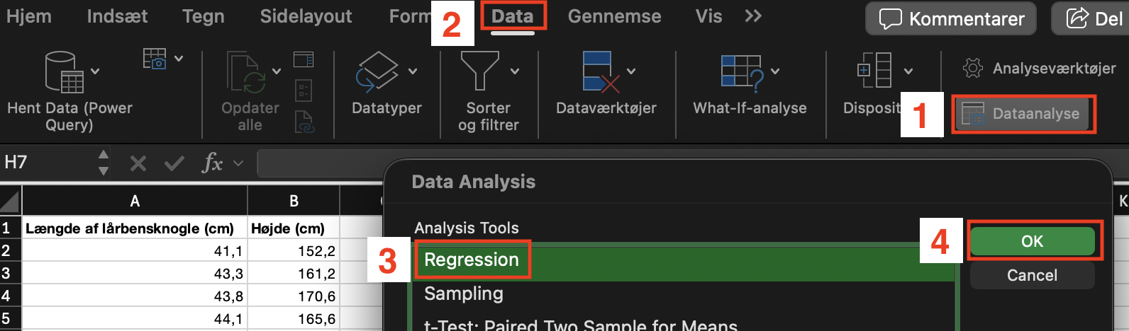
Vi åbner datafilen i Excel og vælger regression under Dataanalyse:
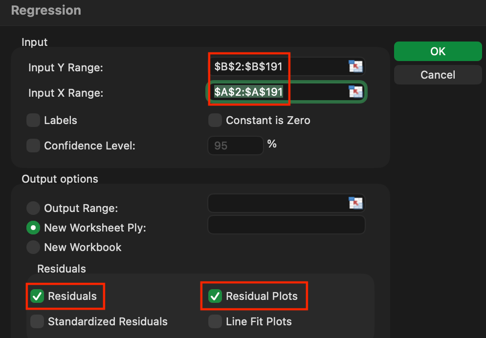
I det næste vindue markerer vi \(y\) og \(x\) værdierne og klikker ”Residuals” og ”Residuals Plots”
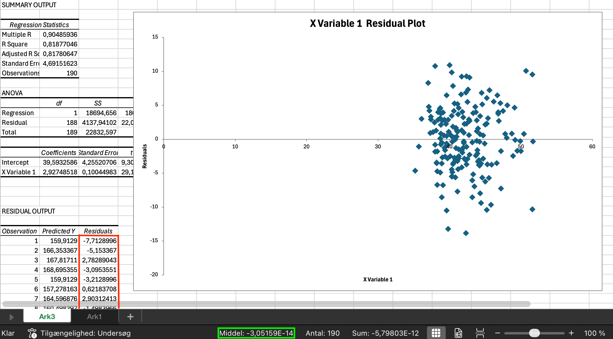
Vi får nu:
Jeg har markeret residualerne og vi kan se, vi får en middelværdi på næsten nul. Vi husker at dette krav automatisk er opfyldt, når vi laver regression på sædvanlig vis.
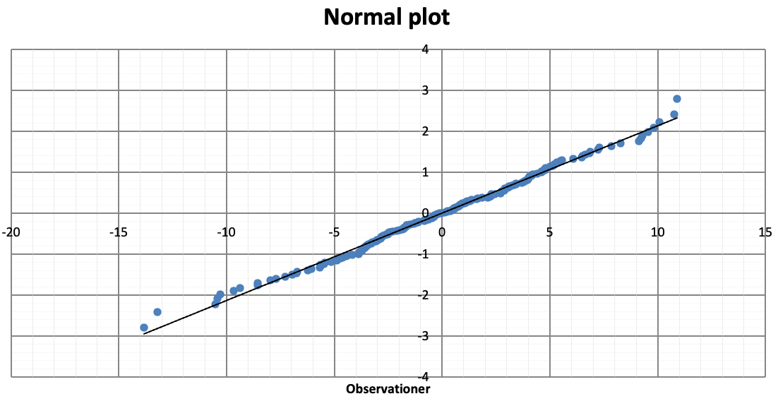
Vi kigger på residualplottet. Det ser pænt ud uden noget tydeligt mønster. Vi copy-paster nu residualerne (markeret med rød) ind i WordMat statistik og laver et normalplot, hvilket giver os:
Vi ser, at punkterne ligger sådan ca. på en linje. Så vi konkluderer, at residualerne er tilnærmelsesvis normalfordelte.
Så vi ser, at residualerne:
-
1. har middelværdi nul,
-
2. ser normalfordelte ud,
-
3. har ensartet spredning omkring linjen fra start til slut (samme varians),
-
4. er uden mønster (uafhængige).
Vi konkluderer, at vores model godt kan bruges.
Øvelse 6.3.1
I eksempel 6.3.1 bliver der lavet modelkontrol af lårbensknogleeksemplet.
Øvelse 6.3.2
Vi vender tilbage til filmdata.
6.3.2
-
a) Vi skal tjekke, at residualerne
-
1. har middelværdi nul:
-
2. ser normalfordelte ud,
-
3. har ensartet spredning omkring linjen fra start til slut (samme varians),
-
4. er uden mønster (uafhængige).
Vi tjekker og får:
-
1. Opfyldt
-
2. Normalplot:
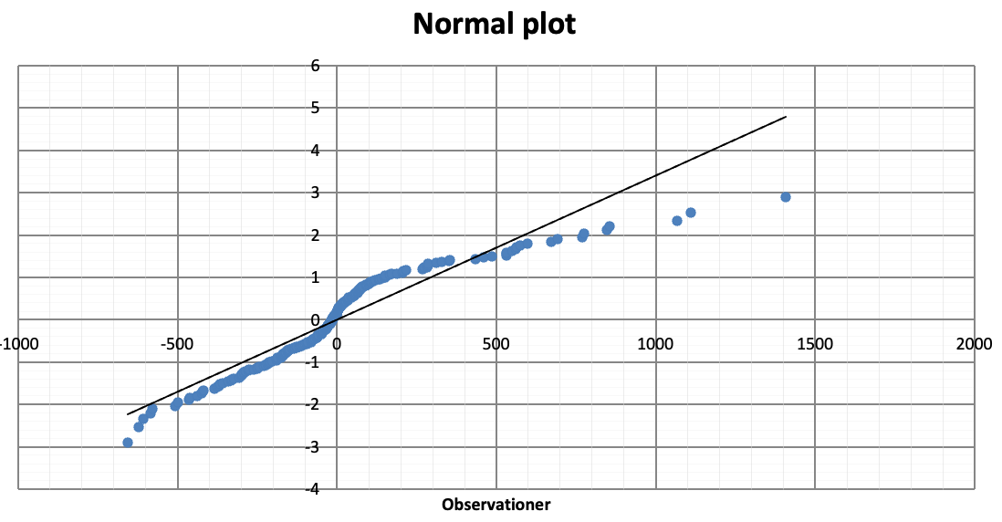
Det ser ud til, at der er systematiske afvigelser fra linjen, så residualerne kan ikke med rimelig siges at være normalfordelte.
-
3. Residualplottet ser således ud:
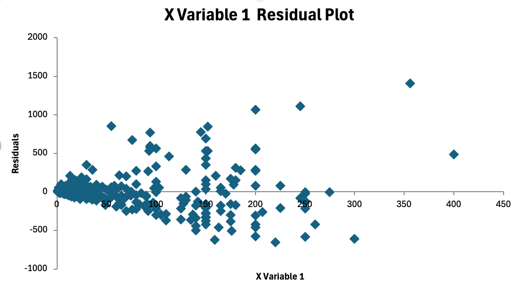
Vi ser at de billige film har mindre varians i residualerne, så kravet er ikke opfyldt
-
4. Ser ok ud.
Alt i alt kan vi konkluderer, at data ikke med rimelighed kan beskrives med en lineær model, og at det konfidensinterval, vi tidligere bestemte, derfor ikke er pålideligt.
Det kan være svært at afgøre, hvornår kravene er opfyldte. Typisk er kravene ikke opfyldt til perfektion, og i praksis er det derfor mere et spørgsmål om, hvorvidt kravene er tilstrækkeligt opfyldt. Det kræver erfaring at vurdere
dette, så hvis du er i tvivl, så beskriv, hvad du mener er problematisk, og at du pga. af dette tager forbehold for modellens validitet.
Outliers
Der kan forekomme observationer som afviger meget for modellen. Dem kan man spotte, når man kigger på residualerne. Der er ikke nogen fast regel for, hvornår man fjerner outliers. Det kan gøres efter forskellige principper. Jeg
anbefaler, at man bruger sin fornuft og fjerner observationer, som vurderes som fejl. Måler man f.eks. temperaturen af vand i en gryde under opvarmning, og en af temperaturene er registreret som \(478^{\circ } C\), så er det nok
fordi at der er skrevet forkert, og derfor bør observationen fjernes fra data.